Single-Epoch Observations

The single-epoch observation preset provides a straightforward way to simulate a measurement as expected by the current reference architecture of LIFE. This includes the generation of synthetic data including instrumental noise, data post-processing, and several tools for signal extraction.

For a detailed documentation of the architecture and the corresponding instrument parameters see the SingleEpochObservation class documentation.

Hint

A public web interface is available for LIFEsimMC, providing access to the GUI for the single-epoch observation preset. See below for more information.

Go to Public Web Interface (Beta)

Running a Single-Epoch Observation

The singe-epoch observation preset requires the specification of the astrophysical scene, including information on the target star, exozodiacal dust, and the observed planet. Additionally, the integration time for the observation must be specified.

Note

For a documentation of all configurable parameters and default values, check out the SingleEpochObservation class documentation.

The easiest way to run a single-epoch observation simulation with LIFEsimMC is through the GUI. This can be done through the public web interface or by running it locally. However, it can also be run in a regular Python script through the Python API.

Graphical User Interface (GUI)

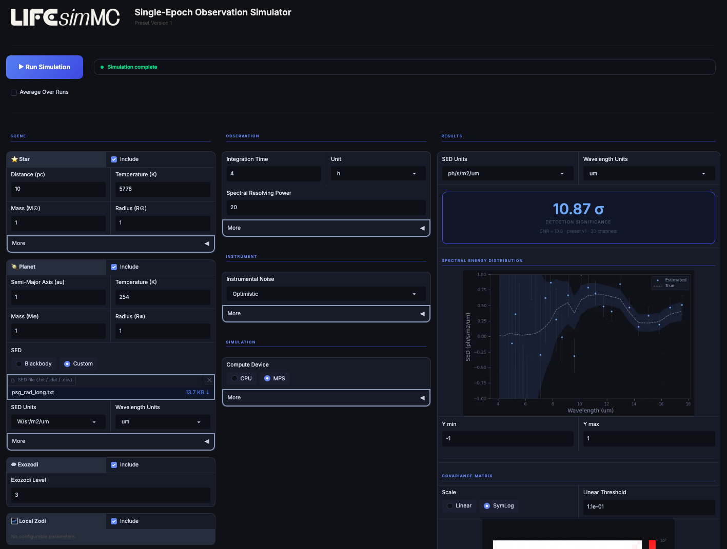
Screenshot of the GUI of the single-epoch observation simulator.

To run the GUI (see screenshot below) locally (after installing LIFEsimMC), open a console and run the following command:

lifesimmc-gui

The single-epoch observation simulator will then be hosted locally on your machine and you can just click on http://127.0.0.1:7861 to open it. Alternatively, you can open a browser and manually navigate to http://127.0.0.1:7861. A screenshot of the GUI is shown in the figure above.

After specification of the astrophysical scene and the integration time (and optionally other parameters), the full simulation can directly be run by clicking the “Run Simulation” button. The estimated planet SED and several other outputs are then displayed in the GUI. All outputs can be downloaded as numpy arrays from within the GUI.

Python API

All results offered by the GUI can also be accessed through the Python API. The following notebook illustrates how to setup the astrophysical scene, run the single-epoch observation and plot all results.

Import Necessary Modules

We start by importing the necessary modules.

import astropy.units as u
import matplotlib.colors as mcolors
import numpy as np
import torch
from matplotlib import pyplot as plt
from phringe.core.scene import Scene
from phringe.core.sources.exozodi import Exozodi
from phringe.core.sources.local_zodi import LocalZodi
from phringe.core.sources.planet import Planet
from phringe.core.sources.star import Star
from phringe.io.sed_loader import SEDLoader

from lifesimmc.lib.instrument import InstrumentalNoise
from lifesimmc.presets.single_epoch_observation.single_epoch_observation import SingleEpochObservation

Matplotlib is building the font cache; this may take a moment.

Define Astrophysical Scene

Next we define the astrophysical scene, consisting of a star, a planet, an exozodi, and the local zodi.

scene = Scene()

# Create star
star = Star(
    name='Sun Twin',
    distance='10 pc',
    mass='1 Msun',
    radius='1 Rsun',
    temperature='5778 K',
    right_ascension='10 hourangle',
    declination='45 deg',
)

# Create planet
earth_twin = Planet(
    name='Earth Twin',
    propagate_orbit=False,
    sed_loader=SEDLoader(
        path_to_file='../_static/psg_earth_spectrum.txt',
        sed_units='W/sr/m2/um',  # Alternatively: u.W / u.sr / u.m**2 / u.um
        wavelength_units='um',  # Alternatively: u.um
    ),
    mass='1 Mearth',
    radius='1 Rearth',
    temperature='254 K',
    semi_major_axis='1 au',
    eccentricity=0.,
    inclination='180 deg',
    raan='90 deg',
    argument_of_periapsis='0 deg',
    true_anomaly='45 deg',
)

# Create local zodi
local_zodi = LocalZodi()

# Create exozodi
exozodi = Exozodi(level=3)

# Add sources to scene
scene.add_source(star)
scene.add_source(local_zodi)
scene.add_source(exozodi)
scene.add_source(earth_twin)

WARNING: UnitsWarning: 'W/sr/m2/um' contains multiple slashes, which is discouraged by the FITS standard [astropy.units.format.generic]

Note that to use auto-generated blackbody spectra instead of a user-provided SED you can simply set sed_loader=None when creating the planet.

Create Single-Epoch Observation Preset

Then we create a single-epoch observation preset object, adding the scene and defining several other parameters, and run it. This will run the data pipeline in the back and generate and process the data for us. For a list of all configurable parameters have a look at the SingleEpochObservation class documentation.

seo = SingleEpochObservation(
    scene=scene,
    total_integration_time=1 * u.d,
    num_reps=1,
    spectral_resolving_power=20,
    instrumental_noise=InstrumentalNoise.OPTIMISTIC,
    device=torch.device('cpu'),
    grid_size=20,  # Better use at least 40
)

seo.run()

Loading setup...
Done

Done
Generating templates...

Done
Applying ZCA whitening...

Done

Note that here we have set num_reps=1. Setting it to a number larger than 1 will run the same observation multiple times, allowing us to take the means of the results for a more robust interpretation.

Get Detection Significance

We can directly get an estimate of the detection significance of the injected planet through the Neyman-Pearson test.

det_sig = seo.get_detection_significance()

det_sig = det_sig.mean()  # Here the mean is taken over only 1 repetition

print(f"Detection significance: {det_sig:.1f} sigma")

Performing Neyman-Pearson test...
Done
Detection significance: 27.0 sigma

Extract Spectral Energy Distribution (SED)

We can now extract the SED of the planet from the simulated observation.

# Specify output units for SED and wavelengths
sed_units_out = 'ph/s/m2/um'
wl_units_out = 'um'

# Extract SED estimate and associated standard deviation and covariance
sed, std, cov = seo.extract_sed(units=sed_units_out)

# For plotting the SED we take the values from the first repetition rather than the mean
sed = sed[0]

# Take means (here only 1 repetition)
std = std.mean(axis=0)
cov = cov.mean(axis=0)

# Get the instrument wavelength bins and the input (true) planet SED
wl = seo.get_wavelength_bin_centers(units=wl_units_out)
sed_true = seo.get_input_sed(units=sed_units_out)

Done

WARNING: UnitsWarning: 'ph/s/m2/um' contains multiple slashes, which is discouraged by the FITS standard [astropy.units.format.generic]
WARNING: UnitsWarning: 'ph/s/m3' contains multiple slashes, which is discouraged by the FITS standard [astropy.units.format.generic]

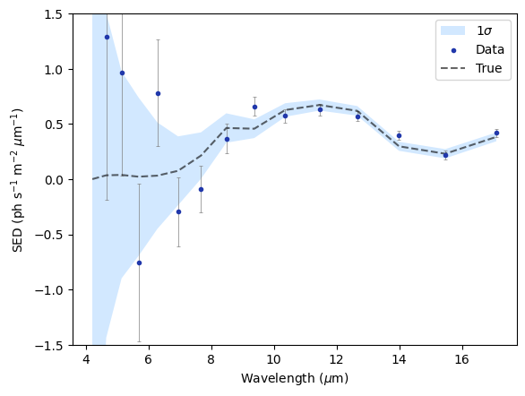
Finally, we plot the simulated measurement:

yerr = np.stack([std, std])
fill_bottom = np.array(sed_true) - np.array(std)
fill_top = np.array(sed_true) + np.array(std)

plt.errorbar(wl, sed, yerr=yerr, fmt='none', ecolor='gray', zorder=1, capsize=1.5, capthick=0.5, linewidth=0.5)
plt.fill_between(wl, fill_bottom, fill_top, color='dodgerblue', lw=0, alpha=0.2, label='1$\sigma$', zorder=0)
plt.scatter(wl, sed, label='Data', color="xkcd:sapphire", zorder=2, marker='.')
plt.plot(wl, sed_true, label='True', linestyle='dashed', color='black', alpha=0.6, zorder=1)
plt.ylabel('SED (ph s$^{-1}$ m$^{-2}$ $\mu$m$^{-1}$)')
plt.xlabel('Wavelength ($\mu$m)')
plt.ylim(-1.5, 1.5)
plt.legend()
plt.show()

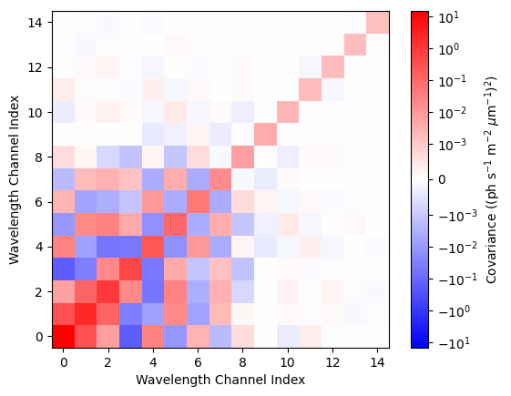
Additionally, we can investigate the estimated covariance matrix:

plt.imshow(cov, origin='lower', cmap='bwr',
           norm=mcolors.SymLogNorm(linthresh=1e-3, vmin=-np.max(cov), vmax=np.max(cov)))
plt.xlabel('Wavelength Channel Index')
plt.ylabel('Wavelength Channel Index')
plt.colorbar(label='Covariance ((ph s$^{-1}$ m$^{-2}$ $\mu$m$^{-1}$)$^2$)')
plt.show()

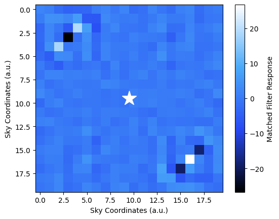
Matched Filter Map

For a visualization of the data we can plot the matched filter map, which we create by comparing the data to a set of planetary templates.

map = seo.get_matched_filter()

# Take the mean over all repetitions
map = map.mean(axis=0)

size = map.shape[1]
center_x, center_y = size / 2, size / 2
import matplotlib.colors as mcolors

hex_colors = ['#000000', '#2749f4', '#4aaaf9', '#FFFFFF']  # Example: red, green, blue
rgb_colors = [mcolors.hex2color(c) for c in hex_colors]
cmap = mcolors.LinearSegmentedColormap.from_list("custom_cmap", rgb_colors, N=256)

plt.imshow(map, cmap=cmap)
plt.plot(center_x - 0.5, center_y - 0.5, marker='*', markersize=21, color='white')
plt.xlabel('Sky Coordinates (a.u.)')
plt.ylabel('Sky Coordinates (a.u.)')
plt.colorbar(label='Matched Filter Response')
plt.show()

Calculating correlation map...
Done

Note

It is recommended to run LIFEsimMC on a GPU, as the simulation gets computationally expensive quickly and may take a substantial amount of time on CPUs.